In this tutorial you will turn an informal claim into a structured argument, entirely inside Visual Studio Code. You will write your first jPipe model, preview it as a live diagram, and export that diagram as an image. By the end of this guide you will be able to:
- Create a justification model in the
.jdformat. - Understand the relationship between evidence, strategies, and conclusions.
- Preview your model as a live diagram, and focus on the part you are editing.
- Export the diagram as an image.
This tutorial only needs the jPipe IDE. If you have not set it up yet, start there and come back.
The scenario: is our release ready?
Imagine you are about to ship version 2.0 of your product. Everyone says it’s ready, but “ready” is vague. jPipe lets you make that claim explicit and back it with evidence.
Let’s make the implicit explicit:
- The goal (conclusion): “Version 2.0 is ready to ship.”
- The reasoning (strategy): “All release gates pass.”
- The facts (evidence): “The test suite passes” and “The changelog is up to date.”
These three roles come from the Toulmin model of argumentation and a simplified Goal Structuring Notation (GSN):
- Conclusion: the claim you want to establish.
- Strategy: the warrant linking the facts to the claim.
- Evidence: the grounds, the concrete facts that support the strategy.
Step 1: Write the model
Create a file named release.jd in the IDE and enter:
justification release {
  // The claim we want to establish
  conclusion c is "Version 2.0 is ready to ship"

  // The reasoning that connects evidence to the conclusion
  strategy s is "All release gates pass"
  s supports c

  // The supporting evidence (grounds)
  evidence e1 is "The test suite passes"
  e1 supports s

  evidence e2 is "The changelog is up to date"
  e2 supports s
}
Every element is declared as <keyword> <id> is "<label>", and support edges (x supports y) wire
the argument together: evidence supports a strategy, and a strategy supports the conclusion.
The // lines are comments. Whitespace is insignificant, and comments help you narrate the
argument. Both C-style forms work:
// a single-line comment

/* a multi-line
   comment */
Step 2: Preview the diagram
With release.jd open, click the magnifier icon in the top-right corner of the editor to open
the live diagram preview beside your code. The preview refreshes as you type.
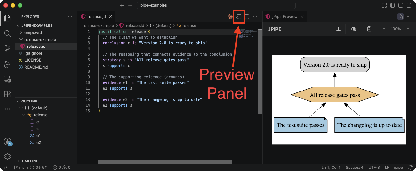
The rendered argument looks like this:

Reading the shapes:
- Conclusions are grey rounded rectangles.
- Strategies are amber hexagons.
- Evidence is shown as blue notes (folded-corner boxes).
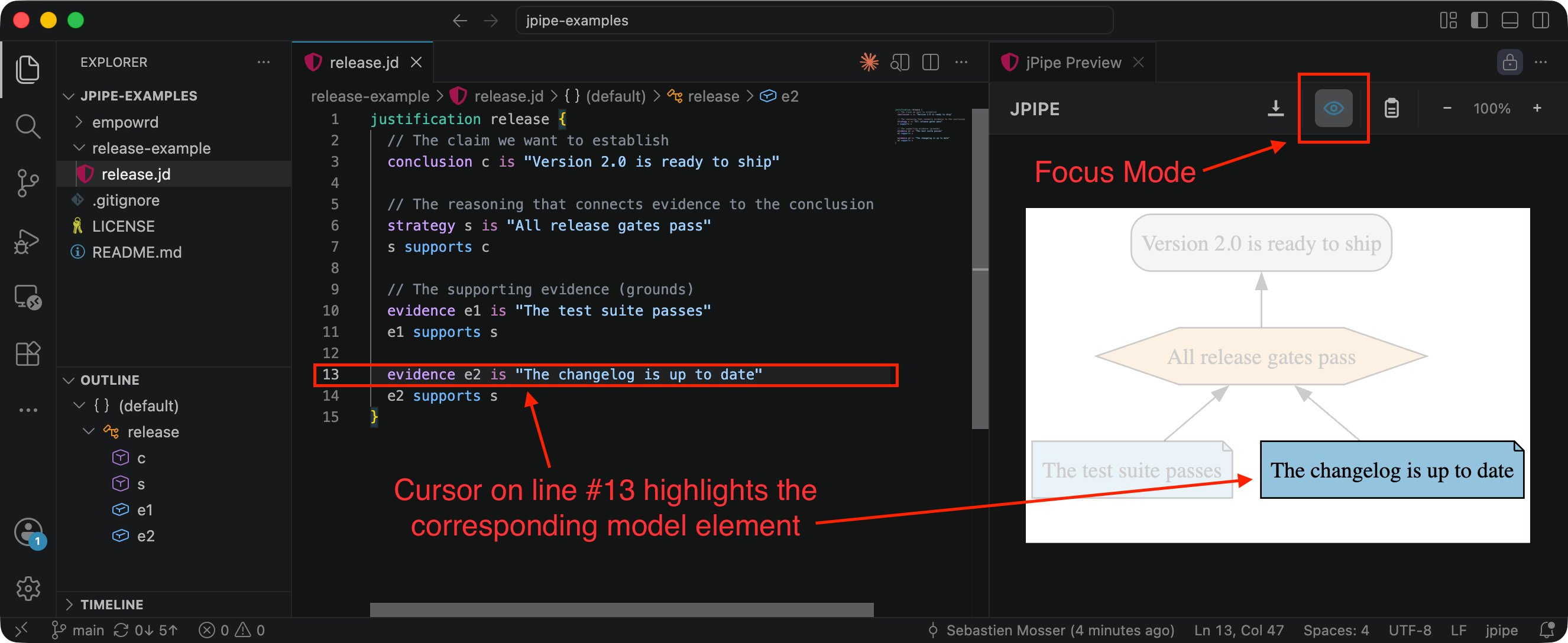
As you move your cursor through the model, focus mode highlights the matching element in the diagram, so you can see which part of the argument each line builds.
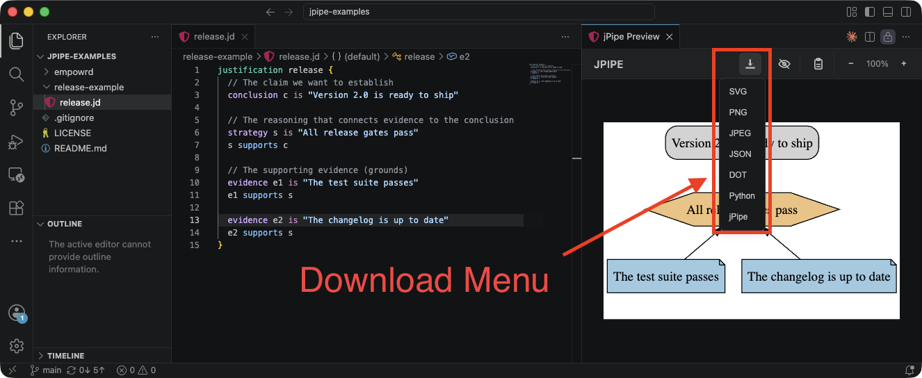
Step 3: Save the diagram as an image
Happy with the result? Use the download menu in the preview to export the diagram as an image, either SVG (vectorial format, crisp at any size), PNG or JPEG.
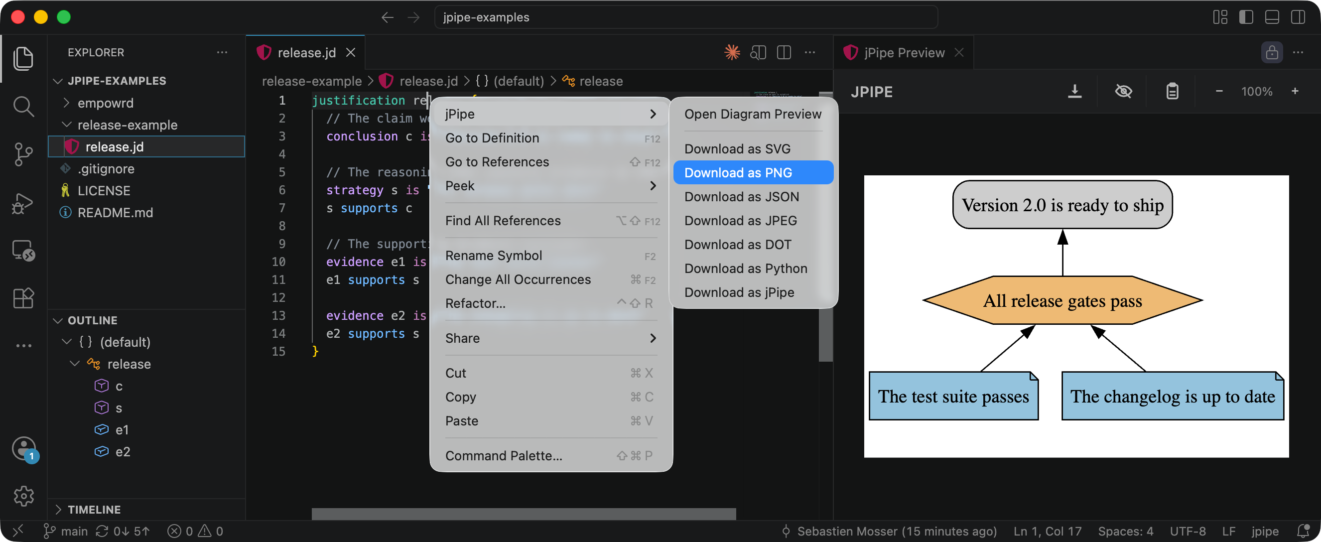
An alternative: the right-click menu
Every jPipe action above is also available from a context menu: right-click anywhere in an open
.jd file and jPipe adds its commands (Open Diagram Preview, Download as SVG/PNG/JPEG, and more)
straight to the menu, so you can reach them without the magnifier icon.
🎉 That’s it: you have written, previewed, and exported your first justification, all from the IDE.
Where to next?
Your first justification is intentionally shallow: a single strategy asserting “all gates pass” with two flat pieces of evidence. Real arguments grow structure, and eventually teeth:
- Sub-conclusions grow the argument with intermediate claims, and splitting models breaks it across files.
- Make it executable binds each piece of evidence to a real check with the jPipe Runner.